
As described elsewhere, understanding a team’s baseline capacity will provide a rough indication of its overall capabilities. This measure can be used to set benchmarks, uncover hidden capacity and generally ensure that resources are being well utilized at a given point in time. What baseline capacity does not do however, is help managers predict future needs or manage long term risk. For that you need to understand the capacity of a team and how that capacity changes over time. We call this the team “velocity”.
A team’s baseline capacity is essentially an optimal view of the team. It is representative of laboratory conditions, though it can be an effective measure to show the impact of a single variable within a specified period of time (i.e. all things remaining equal, if we added one resource the impact would be as follows…). The trouble arises when there are layers of conditions applied on top of the countless variables that could impact production as time moves along. This is the normal operating state for most firms.
Calculating team velocity, or the overall pace of production over time, is a function of the impact of each variable and the conditions that exist at the time. Variables are specific changes to the operating environment that could yield an improvement or decline in current baseline capacity. A condition is an offset to the variable. For example, adding a new resource to a team represents a positive variable in that the new resource will add capacity. However, that capacity will not be consistent over time. Initially the new resource will not be effective from a productivity standpoint and will in fact be a drag on productivity as he/she is using up the capacity of more experienced staff members to assist with training. So, the condition can be a positive or a negative weighting on a variable (or both at different times), in this case the productivity level of a number of resources.
Let’s take the following example. The baseline capacity of a production team is 100 widgets per day per staff member. There are 10 staff members on the team, so management is expecting production of 1,000 widgets per day. Because of an expected increase in orders the firm now needs to produce 10% more widgets, or 1,100 widgets per day. Management approves the hiring of one new employee to account for the increased production requirements. Once the new headcount is approved, the sales team needs to adjust their targets upwards and the finance team will want to know when they can begin to accrue 10% more revenue. The operations manager, in this case in a production role, will need to effectively manage his stakeholder’s expectations as to when the increased production will be available for sale. Only then can adjustments actually be made to accruals and sales targets. To do that he must be able to calculate the team’s velocity over time.
In the model below, the production manager can show several changes in team velocity over time. In fact, he can show a drop in team capacity during the interview process where key production resources are used to help select candidates. Then, after returning to normal briefly, productivity drops again when the winning candidate starts work and resources will again be utilized in a non-production capacity, this time to train the new resource. As the new hire comes up to speed some capacity is regained from the team members who are participating in training as well as by the partial contribution of the new hire. After six weeks of training the team as a whole has returned to its pre-hire production rates. And with a few more weeks of maturity, the new hire is now a fully contributing member of the team and the production target of 1,100 units is achieved and becomes the new baseline.
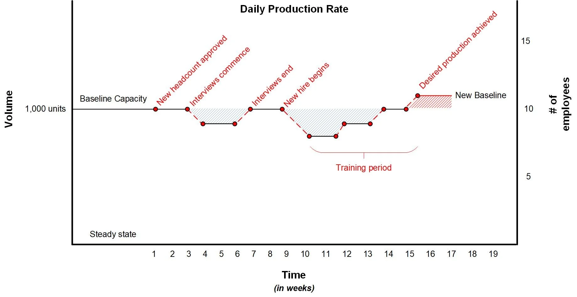
In this example, as in the real world, the production manager has several options. First, he or she can explain to stakeholders and senior management that there will be a short-term hit to production as the team ramps up. That may be acceptable, but if it’s not acceptable then the manager can propose the authorization of overtime or the reallocation of appropriate resources to cover the production gaps (represented as blue hash marks above).
In the end, it will take a total of sixteen weeks and there will be a total of eight weeks of diminished capacity in order to achieve the production goals. If the finance team accrues revenue at the time of the new headcount approval then the overall objectives for the year will likely be off by a quarter.
In the above example, each variable resulted in a change in productivity rates for a period of time. Let’s say the interview resulted in using 20% of two resources for that two-week period between screening, meetings and in-person interviews. Production for that period was reduced because two resources were 20% less effective during that period. When the new person started, those same two resources now dedicated 50% of their time to training, editorial tasks, meetings and other activities required to on-board the new employee. Again, you can see a drop in productivity rates during the training period. Although, as the new employee comes up to speed you can see a stepped improvement in productivity for the team as the two trainers are less burdened by training activities and the new hire begins to contribute positively.
Velocity is the sum of units of work, resources and time increased or reduced by the effect of production variables and the conditions that govern them.

In the above example where two resources were involved in training, the velocity for the team overall in week 10 and 11 would be:
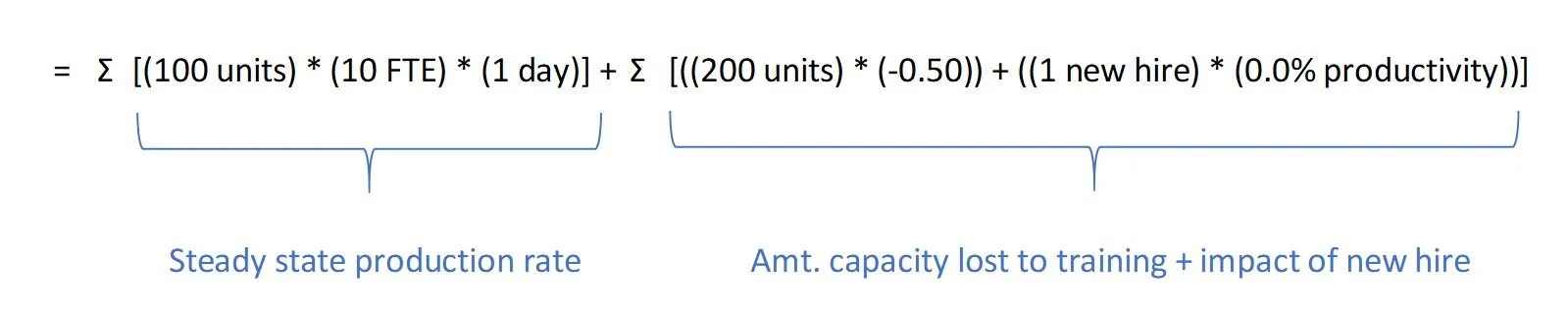
The starting point in the calculation is 100 units 10 full-time employees (FTE) 1 day = 1,000 units per day, or the steady state before the hiring action. In this case, two resources are rendered only 50% effective as production resources because of training activities. In any given day, these trainers would produce 200 units. Now they will only produce 100 units in the period. The new hire in these weeks produces zero capacity. So, the team velocity in this period as depicted as a daily rate would be 900 units and not the requisite 1,000 units.
If this same calculation was produced for each of the impacted periods and then averaged, you would have the overall velocity, or daily pace of production, for the quarter. These values could be used to calculate accruals and sales targets, etc.
For more information about this article or our services, reach out to us at info@coeurderoy.com.